Background and motivation
This workflow emerged from a practical need: maintaining dynamics analysis skills during a career break, using only free tools. Throughout my career as a mechanical engineer, I have emphasised programming competency alongside engineering analysis. My specialisation is dynamics — structural dynamics, mechanism analysis, aeroelasticity — and my standard workflow combined hand derivations, Mathematica for symbolic computation, and MATLAB for numerical methods and simulation.
Four years ago I took a six-month sabbatical to travel. I wanted to keep my engineering skills sharp and set a goal to learn Python. As a project-oriented learner, I looked for a way to apply my existing dynamics skills in a new language. What I found was that sympy covers many of my MATLAB use cases, and scipy covers most of the numerical methods. Both are free and can be launched in a browser through Google Colaboratory without any installation.
sympy.physics.mechanics is a Python module within the SymPy library that provides tools for symbolic derivation of equations of motion (EOM) for mechanical systems. It supports Newton-Euler, Lagrange, and Kane's methods, and handles the time derivatives required to compute velocity and acceleration in systems with complex kinematics.
Why use sympy.physics.mechanics instead of MATLAB?
The practical reasons are cost, accessibility, and standardisation. MATLAB is expensive and requires a licence. SymPy and SciPy are free and open-source, and Google Colaboratory makes them available in any browser.
Beyond cost, sympy.physics.mechanics standardises many of the processes that have been difficult in my career — particularly obtaining time derivatives for velocity and acceleration in mechanisms with complex kinematics, and applying Newton-Euler, Lagrange, or Kane's methods. I have found it useful for classical dynamics problems like pendulums, linkages, and three-dimensional rigid body mechanics. In real jobs I have applied it to actuation load calculations and predicting force or acceleration measurements recorded by test equipment.
| Capability | MATLAB | Python equivalent |
|---|---|---|
| Symbolic math | Symbolic Math Toolbox | sympy |
| Equations of motion | Symbolic Toolbox + manual | sympy.physics.mechanics |
| ODE solving | ode45, ode15s | scipy.integrate.solve_ivp |
| Plotting | MATLAB plot | matplotlib |
| Notebook interface | Live Script | Jupyter / Google Colaboratory |
| Cost | Licence required (~$500+/yr) | Free and open-source |
| Browser-based | No (requires installation) | Yes, via Google Colaboratory |
What is the 8-step sympy.physics.mechanics workflow?
The standard workflow for any dynamics problem using sympy.physics.mechanics has eight steps, which can be applied consistently regardless of system complexity.
- Import required modules —
sympy,sympy.physics.mechanics,scipy.integrate,matplotlib - Define constants and variables — symbolic scalars for mass, length, gravitational acceleration, time, and state variables
- Define reference frames — establish inertial and body-fixed frames; define orientation relationships
- Define positions and velocities — express positions of centres of mass in the inertial frame; compute velocities by differentiating with respect to time
- Define forces and torques — gravity, applied forces, constraint forces
- Apply the equations of motion method — use Lagrange's method, Newton-Euler, or Kane's method to derive the EOM symbolically
- Solve or simulate the ODE — rearrange the EOM into first-order form; use
scipy.integrate.solve_ivpto simulate - Post-process and plot results — extract time histories of states, compute derived quantities, generate plots
Steps outside this Python workflow — such as generating a clear diagram as a starting point — remain part of good engineering practice. More advanced steps, such as 3D mechanics with constraints, may require augmenting the standard transforms with hand-derived expressions.
Worked example: a simple pendulum
A single-degree-of-freedom pendulum is the ideal first example — simple enough to verify by hand, rich enough to show the full workflow and its limitations.
The model is a rigid pendulum link of length L = 1 m, mass m, and moment of inertia I calculated assuming a uniform rectangular aluminium beam (10 cm wide, 1 cm thick). The centre of mass is at half the link length. The angle from vertical is θ with angular rate θ̇. Uniform gravitational acceleration acts downward.
Key symbolic results derived in the workflow include:
- Velocity and acceleration at the centre of the link
- Kinetic energy expression
- Critical angular rate above which the pendulum completes full rotations rather than oscillating (determined to be 7.65 rad/sec in the example notebook)
- The equation of motion, rearranged into first-order ODE form for
solve_ivp
The complete derivation with line-by-line descriptions is available as a Google Colaboratory notebook. The Python portion, stripped to the core sympy sections, fits within the 8-step framework above.
What do the simulation results show?
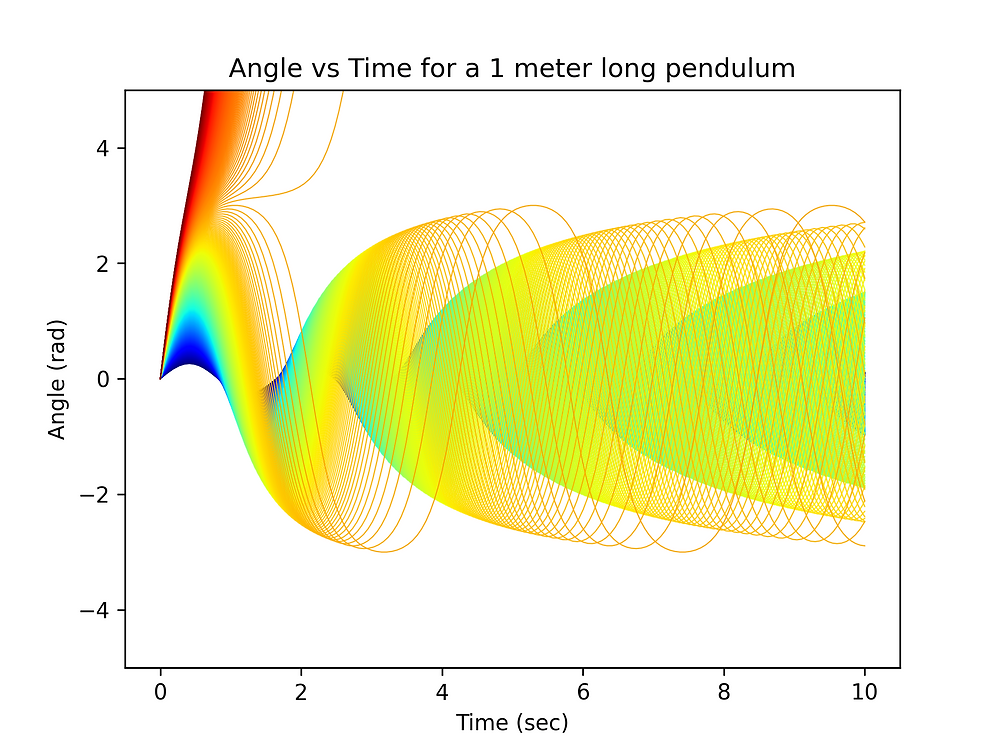
Even with a single pendulum, small changes in initial conditions produce dramatically different responses — which is precisely why this level of analysis matters.
An initial example simulation with an angular rate of 1 rad/sec shows nearly sinusoidal motion with an amplitude of about 0.25 rad (~15°). A broader analysis varies the initial rate from 1 to 10 rad/sec in fine increments:
- Below the critical rate of 7.65 rad/sec: the pendulum oscillates, with oscillation frequency decreasing as the rate increases (the link pauses at its extremes when it passes horizontal)
- Above the critical rate: the pendulum completes full rotations; the frequency increases again, tracking the time per revolution rather than the natural oscillation frequency
Phase plots (angle vs. angular rate) show clear circles for low-rate cases and open trajectories for supercritical cases — a clean verification that the simulation is physically correct.
Conclusion
sympy.physics.mechanics provides an excellent and completely free method for symbolic derivation of equations of motion in mechanism dynamics. The eight-step standardised workflow applies consistently across problems of low-to-medium complexity. I have applied it in real engineering work — linkage and gear train dynamics, actuation load calculations, and as a complement to FEA results. Future posts will cover 3D mechanisms, systems with constraints, and automatic code generation.
Frequently asked questions
Is Python a good replacement for MATLAB in dynamics simulation?
Yes — for symbolic math and equations of motion derivation, sympy.physics.mechanics covers many of the same use cases as MATLAB with Symbolic Math Toolbox. It is free, runs in a browser via Google Colaboratory, and supports Lagrange, Newton-Euler, and Kane's methods.
What is sympy.physics.mechanics used for?
It is used for symbolic derivation of equations of motion in mechanism dynamics. It handles time derivatives for velocity and acceleration in complex kinematics, and is useful for pendulums, linkages, rigid body mechanics, and actuation system analysis.
Can I run Python dynamics simulations for free?
Yes. SymPy and SciPy are free and open-source. Google Colaboratory lets you run Python notebooks in a browser without any installation.
What are the 8 steps in the sympy.physics.mechanics workflow?
Import modules → define constants and variables → define reference frames → define positions and velocities → define forces and torques → apply EOM method (Lagrange/Newton-Euler/Kane's) → solve ODE with solve_ivp → post-process and plot.